| Author | Affiliation |
|---|---|
| Edward J. Lin, MD, MPH | Department of Emergency Medicine, Kern Medical Center, 1830 Flower Street, Bakersfield, CA 93305 |
| Thomas B. Purcell, MD | Department of Emergency Medicine, Kern Medical Center, 1830 Flower Street, Bakersfield, CA 93305 |
| Rick A. McPheeters, DO | Department of Emergency Medicine, Kern Medical Center, 1830 Flower Street, Bakersfield, CA 93305 |
ABSTRACT
Prediction models using multiple logistic regression are appearing with increasing frequency in the medical literature. Problems associated with these models include the complexity of computations when applied in their pure form, and lack of availability at the bedside. Personal digital assistant (PDA) hand-held devices equipped with spreadsheet software offer the clinician a readily available and easily applied means of applying predictive models at the bedside. The purposes of this article are to briefly review regression as a means of creating predictive models and to describe a method of choosing and adapting logistic regression models to emergency department (ED) clinical practice.
INTRODUCTION
Articles reporting clinical prediction models that employ regression techniques are appearing with increasing frequency in the medical literature.1 One of the principal reasons for carrying out a regression analysis is to generate a tool that will help predict an outcome (dependent variable) from available clinical information (independent, explanatory or predictive variables). When validated, such tools may be used to supplement clinical judgment and improve patient care. Comparisons of clinical performance with and without the use of such models support the contention that improved diagnostic accuracy and standardization of care can result from their use in the workplace.2–8
Two major problems associated with predictive models are the complexity of computations associated with their application, and their lack of availability when they are needed at the bedside. Investigators typically modify their derived model to a simplified scoring system using whole numbers. This facilitates calculations, but at the cost of reduced precision of their model, and does not solve the problem of availability.
Use of personal digital assistant (PDA) hand-held devices as a readily available source of medical information is expanding.9 Programs for such devices which incorporate predictive instruments and medical calculators in a “user friendly” format may be downloaded, in many instances for a fee. Unfortunately, such programs are limited in scope and ability to incorporate ongoing changes in medical evidence, and are not easily modified by the user to meet the needs of differing clinical settings.
This article briefly reviews regression as a vehicle for creating predictive models, provides a system for evaluating an article with a predictive model, and describes a relatively simple method for translating the results of studies that use logistic regression (the most common of the regression techniques for creating predictive models) to a PDA spreadsheet format that can be easily applied at the bedside.
Simple Linear Regression
Regression techniques, at their most basic level, employ simple linear regression that describes the straight-line relationship between two variables. A single explanatory (independent) variable (X) is used to predict another (dependent) outcome variable (Y). In the regression model, the slope of the regression line is symbolized by “b”, called the regression coefficient, and “a” denotes the Y-Intercept of the regression line, a constant for that model.
An example of the application of this most elementary form of regression analysis was published by Després et al who examined the ability of waist circumference measurements (in cm) to predict the amount of deep abdominal adipose tissue noted on CT scan (in cm2).10 In their study, waist circumference was the independent variable (X), and the amount of adipose the dependent variable (Y). The regression formula obtained was:
Thus, if the waist circumference of an individual was found to be 70 cm, the predicted amount of adipose on CT was:
Multiple Linear Regression
Many problems in medicine involve multiple predictive variables, all of which must be taken into consideration to predict a single outcome, measured in terms of continuous data, as in the above example. The multiple regression model incorporates two or more independent variables to explain, or predict, an outcome or response. The model, an extension of simple regression, may be represented as follows:
where Y is the dependent (outcome, response) variable, “a” is the intercept of the regression line (a constant for that relationship), X1 is the value of the first independent (predictor) variable and b1 is the regression coefficient associated with it, X2 is the value of the second independent variable and b2 is the regression coefficient associated with it, and so on.
The independent variables typically have continuous numerical values (e.g., weight in kilograms, age in years, etc.). These variables may also have dichotomous (“either/or”) values in which case the presence of that variable is represented by one and its absence by zero. Ordinal values, in which the variable is stratified and ranked in order of increasing severity or exposure, may also be used.
A study published by Benowitz et al illustrates this type of regression analysis.11 They found that the nicotine intake while smoking a cigarette was predictable given the total particulate matter per cigarette and the number of puffs taken. The relation is described by the equation:
where Y is nicotine intake (in mg), X1 is the number of puffs per cigarette, and X2 is the total particulate matter in mg per cigarette, and −0.75 is the constant (intercept) for the model.
With multiple linear regression, while the independent variables may take on dichotomous values, the outcome variable may not. In the frequent case in which the clinician is interested in an outcome with a dichotomous value (e.g., the presence or absence of a particular disease; survival versus death; cure versus treatment failure) the technique of logistic regression is most often employed.
Logistic Regression
In studies using multiple logistic regression the outcome of interest is dichotomous (“either/or” type data) and is expressed within a derived model in terms of the odds that one outcome or the other will occur. Unfortunately, when using odds, the range from zero-chance to even-chance (odds ranging from zero to one) is disproportionate to the range from even-chance to 100% chance (odds ranging from one to infinity). In order to correct for this imbalance, the outcome is expressed in terms of the natural logarithm (ln) of the odds. Ln (odds) can range from minus infinity when the odds are zero, to zero when the odds are one, to positive infinity when the odds are very large. The natural logarithm of the odds is also known as the logit, hence the term logistic regression.
Multiple logistic regression uses the following general formula:
When used in a study seeking to formulate a predictive model, “a” is a constant (analogous to the Y-intercept of the simple linear regression model) generated by the results of the study; b1, b2, b3, and bn are regression coefficients for each independent variable, also generated by the study; and X1, X2, etc. represent the values of each variable for a particular patient. Some authors use α or β0 the regression constant, and β1, β2, etc. to represent the coefficients. Numerical values for the constant (intercept) and the regression coefficients for each variable are often included by the author in the results section. When they are, the reader can reconstruct a formula that will allow precise calculation of probability of outcome, given the values of the variables for a particular patient. This reconstruction of a predictive formula proceeds as follows.
From the above relationship, the ln (odds) of outcome for a particular patient is first calculated by substituting the values for each variable for that patient. Next, by exponentiation, the odds may be found as follows:
where e represents the base of the natural logarithm (equal to 2.71828). Finally, the probability of disease is determined:
Such calculations are impractical for the bedside. However, standard spreadsheet applications created for PDAs may be fairly easily programmed to rapidly carry out these computations as described in the appendix.
SELECTION OF AN APPROPRIATE PREDICTIVE MODEL
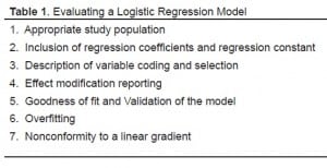
Before adapting a predictive model to the ED bedside, an appropriate model must first be selected and evaluated systematically to ensure the accuracy and proper interpretation of the data. Various guidelines have been suggested for the execution, interpretation, and reporting of multivariate methods. However, as of yet, no consensus exists.12–13 We evaluated the literature, and suggest a set of seven criteria to evaluate a predictive logistic regression model for adaptation to the bedside PDA application (Table 1). We do not propose that if an article does not fulfill all seven criteria it would be deemed unworthy of use in clinical practice. Rather, our goal is to provide a method to evaluate the literature, so that the interpretation of the data and its worth can be appraised by the individual practitioner. The results calculated from the model itself can then be added to the clinician’s fund of knowledge to make a sound clinical decision.
Appropriate study population
When interpreting or applying the result of a study, the study population must be taken into account. For a predictive model to be applied in the emergency department, the study must have a patient population representative of an ED population. This strengthens the external validity of a study, i.e. how generalizable the findings are outside of the study population. Similarly, spectrum bias may distort the accuracy of diagnostic tests and apparent effectiveness of treatments when studied using samples of patients with disease severity more advanced or less advanced, than that in your own clinical population. For example, a model derived from an outpatient medicine clinic or an ICU population may not be applicable to your ED. Examination of the characteristics of the study participants, as well as the inclusion and exclusion criteria must take place, to determine whether the results would be relevant to your patient population.
Inclusion of regression coefficients and regression constant
In order to fully implement the logistic regression model, the regression coefficients and the regression constant (intercept) for the ratios are typically reported, which can be transformed into a regression coefficient by taking the ln(odds ratio), the regression constant is often omitted, making the calculation of probability (the raison d’etre of the model) impossible for the reader.
Description of variable coding and selection
Proper description of the coding of individual variables must be included and examined. The apparent effect of a variable can depend on how the variable is coded. For example, the regression coefficient for the impact of age (independent variable) on long-term mortality (dependent variable) will be different if age is coded in one-year increments versus 10-year intervals, or as a dichotomous variable (less than or greater than 65 years). If a dichotomous (or other categorical) variable is included, the coding method must be replicated to generate accurate results. For example, most authors code presence of the variable as “1” and absence as “0.” Others may use “2” and “1.” The method used by the author must be followed in creating a bedside tool.
Additionally, the reasoning behind selecting independent variables for the model must also be considered, including the level of significance at which the variables were included into the model. An assessment must be made as to whether variables were considered based on prior results, clinical experience, or based on an automated algorithm (“forward” or “backward” selection).12 Proper coding and selection can add to the strength of the result of the model, and thus your clinical practice.
Effect of modification reporting
Interactions between independent variables may influence the coefficients associated with those variables. 12 This interaction, known as effect modification, refers to variation in the magnitude of effect by the variable with varying levels of exposure of another variable.14 Consider, for example, a logistic regression model with lung cancer as the binary outcome variable with two independent (exposure) variables: smoking and asbestos exposure. If the interaction between the exposure variables is not considered, a deceptive regression coefficient estimate for smoking would result. This is because the effect modification of asbestos exposure on smoking is synergistic with respect to lung cancer. When evaluating a model with potential effect modification between variables, mention should be made of the testing for such interactions.
Goodness-of-fit and validation of the model
The validity of inferences drawn from logistic regression techniques depends on the assumptions of the model being satisfied. A critical step in assessing the appropriateness of a logistic regression model is to examine how well the model describes the observed data.15In other words, if an estimate of the outcome is calculated using the model, how well does this estimate “fit” with an actual patient with similar characteristics from the dataset? This is known as “goodness-of-fit,” and is measured by various indexes, including the Hosmer-Lemeshow statistic or reporting of a percentage of the dependent variable that was correctly identified by the model. 16
Validation or retesting of a model in a population different from that used in creating the model is especially important with predictive models to assess model success outside of the derivation study population.12 Internal validation, using the “jackknife” or “bootstrap” procedures, perform the analysis on subsets of the data used to derive the model, investigating the stability of coefficients and predictive ability of the model.12 A better method includes validation analysis on a separate subset of patients not used in the creation of the model. Most desirable is external validation of the model in a population independent of and external to that used in deriving the model, preferably at a separate institution. Reporting of any of these techniques is essential in assessing the validity of model being evaluated.
Overfitting
Overfitting implies that the model has been so refined to conform to the study sample that it has lost general usefulness in application to different populations. A model must have enough outcome events per independent variable in order to have a reliable estimate of risk. Though controversial, studies having fewer than 10 outcome events per independent variable may result in questionable accuracy.16 With overfitting, the resulting regression coefficient may represent spurious associations, or the effects may be estimated with low precision.12
Nonconformity to a linear gradient
In logistic regression modeling, while the dependent variable is binary (dichotomous), the independent variable may be ordinal or even continuous. When a regression coefficient is established for an independent variable, the assumption is that the relationship between the variable and the outcome is linear in nature. That is, a unit change in that variable should always have the same effect on the outcome, regardless of where that unit change occurs in the range of that variable. This may be a problem if the independent variable does not act according to a linear gradient. As an example, the impact of left ventricular ejection fraction on mortality depends not only on the unit change in ejection fraction, but also where the baseline ejection fraction stands. A decrease of 10%, from 30% to 20%, carries greater risk than a decrease from 50% to 40%.12 An article should report the evaluation of conformity to a linear gradient for such variables. Not doing so may overestimate or underestimate the effect depending on the value for an independent variable.
Example
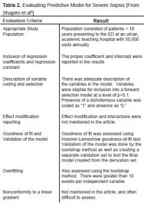
An example below is taken from an article by Shapiro et al,8 which describes a model for predicting 28-day hospital mortality among septic patients based on nine independent dichotomous variables available in the emergency department. Our evaluation of the clinical model based on our seven criteria can be found in Table 2. The study did meet the majority of criteria. The basics of setting up the PDA spreadsheet can be found in the appendix. The variables and their associated coefficients were as follows:
| Variable | Coefficient (b) |
|---|---|
| Terminal illness (<30 days) | 1.80 |
| Tachypnea or hypoxia | 0.98 |
| Septic shock | 0.98 |
| Platelets <150,000/mm3 | 0.93 |
| Bands >5% | 0.82 |
| Age >65 | 0.77 |
| Lower respiratory infection | 0.66 |
| Nursing home resident | 0.62 |
| Altered mental status | 0.50 |
The value of the constant (a) for their model was −5.45.
The logistic regression formula can be reconstructed as follows (taking care to enter plus and minus signs accurately):
Recall that the presence of a dichotomous independent variable in this study was designated by the value 1, its absence by the value 0. For example, if a patient had tachypnea, was in septic shock, had bands of >5%, was 68 years old, had clinical pneumonia and was a nursing home patient (other variables being normal), the calculation becomes:
Setting up this predictive model on a PDA spreadsheet can be found in the appendix.
DISCUSSION
The frequency of use of multivariable methods in the medical literature has steadily increased over the years. One study revealed an 8% increase over a five-year period between 1985–1989.12 Computer-assisted predictive tools as described in this article offer several potential benefits to take advantage of this trend. The results of investigations that produce predictive models may be directly translated into clinical practice without alteration, thereby maintaining their original precision. Physicians using PDAs may be more likely to use the tools when they can be easily tailored to their clinical practice.9Using widely available spreadsheet software, newly validated models may be quickly translated into a form that can be used at the bedside (see appendix), without waiting for third-party software creation and distribution.
There are some important limitations regarding predictive tool adaptation to PDAs. First, predictive models yield only a probability of outcome (e.g., risk of disease, likelihood of benefit from therapy). Establishing thresholds for purposes of diagnostic and therapeutic decision making is a matter of clinical judgment.
Second, a prediction model should be evaluated carefully before it is used in any form. However, proper evaluation is often limited by poor reporting by the author. Bender et al investigated logistic regression in several journals (BMJ, JAMA, the Lancet, and the New England Journal of Medicine) from 1991–94. They found that goodness-of-fit was rarely assessed. Of 111 papers, only seven papers reported a valid assessment of the adequacy of their regression model.17 Other studies have shown similar need for improvements in the reporting and perhaps conducting of multivariable analysis.12 Violations included overfitting of data, a lack of testing for conformity of variables to a linear gradient, no report of testing for interactions, and unspecified coding or selection of independent variables. In the critical care literature, 65% of published articles properly reported coding of pertinent independent variables; 12% referenced whether effect modifications were examined; 1% tested for colinearity; 16% included a goodness-of-fit analysis; and 39% may have overfitted the model, leading to potentially unreliable regressioncoefficients16 In the obstetrics and gynecology literature 51.8% of articles inadequately described the process of variable selection, 85.1% did not report assessment of conformity to linear gradient, only 6.8% tested for goodness-of-fit, and interactions between variables were not assessed in 86.4% of articles.13
Part of the problem with the application of multivariate statistical methods is proper understanding by the study author of these procedures. To this end, editorial guidelines for reporting would improve the ability to interpret a study. If strict reporting guidelines were in place, the methodological flaws in a particular study as well as limitations of model output could be better appreciated.18 Detailed and complete reporting and peer review of such research as well as informed analysis by the clinician evaluating the paper is necessary. The publication of study alone should not ultimately prompt a change in your clinical practice without proper examination of that study.
PDA spreadsheets formatted as predictive tools have been used successfully within our residency for over five years. Our residents have found this to be an effective way to incorporate evidence-based medicine into daily clinical practice. Once created, these tools can be readily shared with other physicians and are easily modified and/or updated as new research is published.
Footnotes
Submission history: Submitted June 22, 2007; Accepted November 8, 2007.
Full text available through open access at http://escholarship.org/uc/uciem_westjem
Address for correspondence: Edward J. Lin, M.D., M.P.H., Dept. of Emergency Medicine, Kern Medical Center, 1830 Flower Street, Bakersfield, CA 93305
Email: edward.lin.uvm@gmail.com
Conflicts of Interest: By the WestJEM article submission agreement, all authors are required to disclose all affiliations, funding sources, and financial or management relationships that could be perceived as potential sources of bias. The authors disclosed none.
REFERENCES
1. Altman DG. Statistics in medical journals: developments in the 1980s. Stat Med.1991;10:1897–1913. [PubMed]
2. De Dombal FT, Leaper DJ, Horrocks JC, Staniland JR, McCann AP. Human and computer-aided diagnosis of abdominal pain: further report with emphasis on performance of clinicians. Brit Med J. 1974;1:376–380. [PMC free article] [PubMed]
3. Teicher I, Landa B, Cohen M, Kabnick LS, Wise L. Scoring system to aid in diagnosis of appendicitis. Ann Surg. 1983;198:753–759. [PMC free article] [PubMed]
4. Pozen MW, D’Agostino RB, Selker HP, Sytkowski PA, Hood WB. A predictive instrument to improve coronary-care-unit admission practices in acute ischemic heart disease. N Engl J Med. 1984;310:1273–1278. [PubMed]
5. Knaus WA, Draper EA, Wagner DP, Zimmerman JE. APACHE II: a severity of disease classification system. Crit Care Med. 1985;13:818–829. [PubMed]
6. Baxt WG. Use of an artificial neural network for the diagnosis of myocardial infarction.Ann Intern Med. 1991;115:843–848. [PubMed]
7. Watts CM, Knaus WA. The case for using objective scoring systems to predict intensive care unit outcome. Crit Care Clin. 1994;10:73–92. [PubMed]
8. Shapiro NI, Wolfe RE, Moore RB, et al. Mortality in emergency department sepsis (MEDS) score: A prospectively derived and validated clinical prediction rule. Crit Care Med. 2003;31:670–675. [PubMed]
9. Barrett JR, Strayer SM, Schubart JR. Information needs of residents during inpatient and outpatient rotations: identifying effective personal digital assistant applications.AMIA Annu Symp Proc. 2003;2003:784. [PMC free article] [PubMed]
10. Despres JP, Prud’homme D, Pouliot MC, Tremblay A, Bouchard C. Estimation of deep abdominal adipose-tissue accumulation from simple anthropometric measurements in men. Am J Clin Nutr. 1991;54:471–477. [PubMed]
11. Benowitz NL, Jacob P, Denaro C, Jenkins R. Stable isotope studies of nicotine kinetics and bioavailability. Clin Pharmacol Ther. 1991;49:270–277. [PubMed]
12. Concato J, Feinstein AR, Holford TR. The risk of determining risk with multivariable models. Ann Intern Med. 1993;118:201–210. [PubMed]
13. Khan KS, Chien PF, Dwarakanath LS. Logistic regression models in obstetrics and gynecology literature. Obstet Gynecol. 1999;93:1014–1020. [PubMed]
14. Rothman KJ, Greenland S. Modern Epidemiology. 2. Philadelphia: Lippincott-Raven; 1998.
15. Hosmer DW, Taber S, Lemeshow S. The importance of assessing the fit of logistic regression models: a case study. Am J Public Health. 1991;81:1630–1635.[PMC free article] [PubMed]
16. Marc Moss D, Andrew Wellman, George A. Cotsonis. An appraisal of multivariable logistic models in the pulmonary and critical care literature. Chest. 2003;123:923–928.[PubMed]
17. Bender R, Grouven U. Logistic regression models used in medical research are poorly presented [letter] BMJ. 1996;313:628. [PMC free article] [PubMed]
18. Carlos VR, Brown MD, George C, Velmahos MD. Clinician or Statistician? Chest.2003;123:677–678. [PubMed]
APPENDIX
PDA Spreadsheet Applications
This section provides a step-wise method for adapting a predictive model, derived using multiple logistic regression, to an easily applied spreadsheet format. The following discussion and examples use formula syntax contained in Documents To Go® spreadsheet software designed for Palm® OS systems.
-
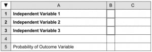
First, a simple spreadsheet is formatted (Figure 1). The darkly outlined cells in column B indicate the areas for data entry by the user. The cells in column C will be used for entering formulae which carry out calculations used in arriving at the final probability of the outcome, contained (in this case) in cell C5. (In the following discussion, cell addresses will be referred to using capital letters, e.g., “C1”, “B2”, etc. Regression constants and coefficients will be referred to using lower case letters, e.g., “a”, “b1”, “b2”, etc.) The formulae used for these calculations take advantage of the “IF” function standard to most spreadsheet applications. This function takes the following general form:
This function prompts the program to first evaluate the condition you specify within the formula. If the terms of the condition are met, then action 1 is carried out; otherwise action 2 is carried out. The results of the action are then entered in that cell. An action may be simply a value, in which case that value is entered in the cell.
Use of the “IF” function allows for simplified data entry, especially when using dichotomous variables. Data entered in the outlined cells may also be continuous (e.g., lab values, weight, blood pressure, etc.) or ordinal (multiple ranked categories). Note that units are not entered in the data entry cells, only numerical values.
Dichotomous predictive variables are generally given a value of 1 if present and a value of 0 if absent. However, using the formulae below further simplifies data entry in thatany character (e.g., an “x”) placed in the appropriate cell in column B is taken as 1; if no character is in the cell in column B then the value is taken as 0. The appropriate value is then multiplied by the regression coefficient for that variable and the result is automatically placed in the cell. For example, for the three variables in the sample spreadsheet, the following formulae could be entered:
The above formulae take advantage of the spreadsheet’s ability to distinguish an empty cell from one with a character contained in it. The “< >” indicates “not equal to” and the double quotes (with no space between them) denote an empty cell. The symbol “*” denotes multiplication. These expressions can be more simply written as:
In plain terms, the last formula (in cell C3) instructs the program to do the following:
“Evaluate cell B3. If it is not empty (i.e., contains a character) then enter the value for b3 (the regression coefficient for that variable) in cell C3. Otherwise, if cell B3 isempty, enter a zero in cell C3.”
With the above formulae entered in cells C1, C2 and C3, if an “x” is entered in cell B1, then the value for b1 is automatically entered in cell C1. If the “x” is removed from cell B1, a zero is entered in cell C1.
If the value for the third variable were continuous, then the following formula would be entered in cell C3:
This instructs the program that if a numerical value is entered in cell B3, that value is to be multiplied by its regression coefficient and the result entered into cell C3. If no value is present in cell B3, then a zero is entered in cell C3.
-
Returning to our basic formula:
Ln(odds) outcome = a + (b1)(value of variable 1) + (b2)(value of variable 2) + (b3)(value of variable 3) = a + C1 + C2 + C3 This formula may be entered in cell C4 as follows:
where “a” is the regression constant, hopefully also supplied by the author. (The term “C1:C3” is spreadsheet shorthand signifying “all the cells in column C, from C1 to C3, inclusive.”)
The value calculated in cell C4 is equal to the natural logarithm of the odds of the outcome variable, i.e.:
-
Next, taking the antilog of each side of the equation yields:
and since the antilog of the logarithm of a number is the number itself:
which is equivalent to:
In the language of the spreadsheet, the natural antilog of term x is found by the formula:
or, for our example:
-
To convert odds to probability, use the relationship:
As a shortcut, steps 3 and 4 above can be combined in cell C5 as the following expression:
This calculation in cell C5 yields the probability of disease, given the presence or absence of the independent variables listed. It is expressed in decimal form. To convert it to percentage, simply reformat the cell to percentage format.
Example
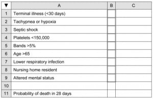
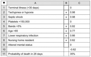
Using our example from the article by Shapiro, et al,8 setting up the predictive model on a PDA spreadsheet proceeds as follows. First, create the layout as shown in Figure 2. Enter the following formulae in column C (recall that the “< >” indicates “not equal to” and the double quotes denote an empty cell):
Now, when the user enters an “x” in the appropriate data entry cells, the values for this patient would appear as shown in Figure 3.


