
| Author | Affiliation |
|---|---|
| Joshua C. Chang, MS | University of California, Los Angeles, Department of Statistics |
| Frederic P. Schoenberg, ScB, PhD | University of California, Los Angeles, Department of Statistics |
ABSTRACT
Ambulance response times in Santa Barbara County for 2006 are analyzed using point process techniques, including kernel intensity estimates and K-functions. Clusters of calls result in significantly higher response times, and this effect is quantified. In particular, calls preceded by other calls within 20 km and within the previous hour are significantly more likely to result in violations. This effect appears to be especially pronounced within semi-rural neighborhoods.
INTRODUCTION
The importance of rapid ambulance response to emergency medical crises has been well-documented. Indeed, after early access, early cardiopulmonary resuscitation (CPR), and early defibrillation, early access to advanced care is the fourth and final link of the Cardiac Chain of Survival,1 according to the American Heart Association. While a study in Ontario, Canada concluded that to improve survival rates after cardiac arrest, ambulance response times must be reduced and the frequency of bystander-initiated CPR increased,2 a subsequent study found that system wide implementation of full advanced life support programs had a negligible impact on mortality among victims of major trauma.3 A study performed in King County, Washington determined the survival rate to decrease by 2.1% per minute without intervention by advanced cardiac life support (ACLS).4 When urban response time was correlated with myocardial infarction survival rate in a Southwestern metropolitan county with a population of 620,000 a response time of under five minutes was found to have a beneficial impact on survival.5 Similarly, studies have shown that response time and transport time are correlated with survival rates for abdominal gunshot wound victims, and that the overall total emergency medical services (EMS) pre-hospital time interval was significantly lower for trauma survivors than for non-survivors.6,7
While any decrease in ambulance response time is likely to be beneficial, several studies have taken the approach of spatial-temporal modeling of response times to highlight particular areas where heightened efforts toward improved response may be especially desirable. For instance, a study in Houston, Texas used a queueing model to show that increased dispersion of ambulances in areas away from those of high demand improves the tail of the response time distribution.8 Similarly, a computer-based model developed for Los Angeles County was able to reliably predict response time and search for an optimum pattern of ambulance deployment to minimize mean response time as well as response time excesses.9
The focus of this paper is the retrospective analysis of the spatial-temporal pattern of response times in Santa Barbara County, California in 2006 with particular attention to the impact of the number of spatial-temporally proximate emergency calls on response times. Our goal is to investigate the dependence of ambulance response time on system load, to identify particular areas where improvements might have the most effect. For a fixed region with a finite number of ambulances, one may anticipate that response times may increase during times when a substantial portion of the ambulances are unavailable due to previous emergencies.
METHODS
Data
Santa Barbara County consists of three geographic service areas. Each area is further divided into zones dependent upon population density. The fire department provides basic life support (BLS) first response within the two-tiered response system. ALS response and transport is contracted out to various ambulance companies. Santa Barbara has adapted ambulance response-time regulations dependent upon population density (Table 1). The county operates on a base hospital system with each geographically defined base hospital providing all field medical direction. All approved hospitals in the county are designated base hospitals.
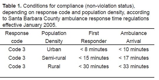
Response-time regulations effective January 2005 provided standards for the timeliness of an ambulance response given its response code and the population density of the area to which it is responding. From these regulations it was determined whether each dispatch event was in compliance with the standard, or whether it was a violation, i.e. an exceedance of local response-time standards.
County ambulance dispatch data for 2006 were provided by Santa Barbara’s EMS agency for the UCLA Statistics Department’s EMS study group, and this study was approved by the agency’s director. As measures of ambulance response performance, both response time and response-time regulation compliance were used, with ambulance response times defined as the time elapsed between ambulance dispatch and ambulance on scene arrival. Events for which ambulance response time could not be determined due to missing data were excluded. Events where the location could not be determined are excluded from analysis as well. Since the focus of this study is on emergency calls, analysis of Code 3 dispatched calls (ambulance response with lights and sirens)10 was emphasized, but other calls were considered as well since they are drawn from the same resource pool.
Data Analysis
Our analysis uses existing tools for analyzing spatial data. The spatial call distribution was estimated non-parametrically using kernel intensity estimation,11,12,13 which involves smoothing the data and interpolating values between observations by averaging nearby values, weighting them by distance. Logistic regression14 was used to investigate the relationship between the number of calls closely preceding any given incident and the percentage of violations. One aim of the present study is to look for evidence of spatial clustering of violation incidents, and in particular for clustering of violation incidents that had a positive number of preceding calls, and the inhomogeneous K-function15,16 was used for these purposes.
Methodological Details
The R Language and Environment for Statistical Computing17 was used to perform data management, Fisher’s exact test, multiple comparisons, and spatial analyses. Variables recorded include the incident time, geographical address, incident type, response code, response district, response district type, ambulance dispatch time, ambulance on scene time, hospital arrival time, and incident clear time. The addresses were geo-coded by the EMS study group into longitude and latitude coordinates and subsequently transformed into more natural units of kilometers using the Universal Transverse Mercator coordinate system.
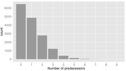
As a measure of system load at the time of each call, we define the statistic β for each call, as follows: If {(ti, xi); i = 1, …, 21,944} represents the collection of times (ti) and locations (xi) of recorded calls, let βi (Δt, Δx) = ∑j<i 1 {ti − tj ≤ Δt} 1 d(xi, xj) ≤ Δx}, where 1 denotes the indicator function, and d(xi, xj) denotes the spatial distance between locations xi andxj. Thus βi (Δt, Δx) represents the number of calls prior to call i that were within Δt hours and within Δx km of call i; such calls are subsequently referred to as predecessors of call i.
After many choices of the parameters Δt and Δx were inspected, particular attention was focused on the case where Δt = 1 hour and Δx = 20km, which appears to have the highest correlation with response time. The parameter Δx may be interpreted as an approximation of the average area of an ambulance dispatch region, while a possible interpretation of Δt may be the mean time required for an ambulance to return to service after it has been dispatched to a previous call.
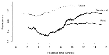
To see how variation in the number β of predecessors is associated with response time, the incidents were first blocked for response code and district type. Within each block, the relationship between β and response time was smoothed using simple moving average (MA) filtering.18
If M represents the total number of ambulances available for service in a particular area, and k represents the number of ambulances that are actively responding to incidents, then M-k is the number of ambulances in service that are available to respond to new calls. One would expect response time to depend less heavily on k in regions where M is larger. Similarly, in such regions, one would anticipate a one-unit increase in β to be associated with a smaller increase in mean response times for such regions.
A one-sided Fisher’s exact test was used to determine whether the proportion of violations was significantly greater for incidents where β>0, compared with incidents where β=0. The relationship between the number of predecessors and the probability of a violation was summarized using logistic regression.14
The spatial call distribution was estimated non-parametrically using kernel intensity estimation, with an edge-corrected, isotropic Gaussian kernel.11 Due to geo-coding precision inaccuracies, 24 call incidents lay outside of Santa Barbara County boundaries; for the kernel intensity estimate, these points were excluded.
The inhomogeneous K-function15 was used to measure spatial clustering of violation incidents and of violation incidents that had a positive number of predecessors. The inhomogeneous K-function may be used as a measure of the degree of clustering or inhibition in points above and beyond what one would expect from a baseline model.16Here, we used the kernel estimate of the call rate at each location, scaled by the proportion of calls in violation, as a baseline model. Since many of the points in the data set lie near the county borders, the choice of edge correction technique may have a substantial impact on the estimated inhomogeneous K-function, so standard edge-correction methods were used.11,12
To identify areas where β shows more of an effect on the proportion of violations, the fraction of calls that were violations among calls with predecessors was compared with the same fraction among calls without predecessors, for each spatial-temporal sub-region. This difference was computed for all calls within a bandwidth λ around each incident, provided there were at least 10 incidents within a distance of λ. As with other smoothing procedures, the bandwidth λ should be chosen to be sufficiently small so that local detail is detectable, but large enough so that main features are not obscured by local fluctuations.11 Contours were drawn around regions where the difference in proportion of violations was 5% or greater for Code 3 calls. These areas reflect regions that might benefit the most from increased ambulance units or from optimizing the deployment pattern of existing ambulances.
An exponential distribution was fitted to the distribution of incident inter-arrival times, which are defined simply as the elapsed time between each incident and the event preceding it. The exponential distribution for inter-arrival times is consistent with a time-homogeneous Poisson process for call arrivals. As an alternative to the time-homogeneous Poisson process, we considered an inhomogeneous Poisson process with the temporal rate given by a kernel density estimate of the call times.
All multiple hypothesis testing was performed controlling family-wise error rate at α = 0.05 using Holm’s stepwise p-value correction.18
RESULTS
Of the 21,944 recorded emergency ambulance dispatch events in Santa Barbara County in 2006, 15,883 (72.4%) were Code 3 responses. Of these, 14,199 (89.4%) ambulances were to urban zoned areas, 1,382(8.7%) to semi-rural zoned regions, and 302(1.9%) to rural regions. Overall, 97.4% of Code 3 ambulance responses had response times within legislated limits.
For calls where β=0, i.e. calls without predecessors within one hour and within 20 km, the proportion of response time violations was 2.96%, whereas for calls with β>0, the proportion of violations was 4.56%. The increase in probability of violation associated with having predecessors is highly significant (Fisher’s exact test; p = 7.2 × 10⁻¹⁰). As β increases, both the response time and the probability of a response time violation were seen to increase. The fit of a logistic regression model to the relationship between violation and β implies that on average, for each additional predecessor, the log odds ratio log{p ÷ (1−p)} of the probability of violation increased by 19.1% (p = 6.3 × 10⁻¹¹). The increase in response time associated with increasing β is seen in Figure 2, which shows the response time as a function of number of predecessors, smoothed using a moving average (MA) filter. The positive association between β and response time across different response codes and population densities is evident in Figure 2. However, the difference in probability of violation associated with changing β is seen to vary across response codes and district types. The increase in proportion of violations is most pronounced in semi-rural calls.
Overall, the inter-arrival times between calls follow approximately an exponential distribution with a rate of 2.51 calls per hour. The rate of call arrivals seems to vary, however, according to the time of day, the highest frequency of calls were at mid-day. Indeed, the frequency of calls between 9 am and 6 pm is approximately three times higher than that between 2 am and 6 am. Not surprisingly, the proportion of calls where β>0 varies according to the time of day as well. A multiple-comparison one-sided Fisher’s exact test shows that for the hours of 9am–10am, 12pm–1pm, 5pm–6pm, 8pm–9pm, and 10pm–11pm, there is a statistically significantly higher proportion of calls that have predecessors. The difference in proportion of calls that were violations for β=0 and β>0 varies according to the hour of day as well with the highest proportion between 6am–7am and between 5pm–6pm, perhaps due to traffic incidence. We then categorized the calls according to whether β=0 by hour. We found that between 6am and 8am, 5pm–6pm, 8pm–9pm, and 11pm–11:59 pm, the proportion of calls with β > 0 that are violations is much higher than that for calls with β = 0. By contrast, during other hours the proportions are similar, and between 4am and 5am, the proportion of calls that are violations is actually higher for calls without predecessors than for calls with predecessors, perhaps due to lack of available personnel.
The spatial distribution of ambulance response events consists of several areas of high concentration, surrounded by vast areas of very low concentration, within the 9,814 km2 that comprise Santa Barbara County. Figure 3 shows a kernel intensity estimate of the spatial call rates. One sees that the vast majority of calls are clustered within the main urban parts of Santa Barbara County, especially in the cities of Santa Barbara, Carpinteria and Goleta (in the southeast), with one cluster in Santa Maria (in the northwest), and another in Lompoc (toward the southwest).

Using the inhomogeneous K-function, one can assess the extent to which the observed points exhibit significant clustering beyond what one would expect from an inhomogeneous Poisson process. The inhomogeneous K-function, for calls which were in violation and which had a positive number of predecessors, is shown in Figure 4.
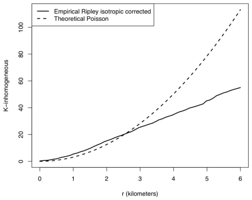
It is clear from Figure 4 that there are areas where violations are more likely to coincide with predecessors than expected under the null hypothesis that the violations occur according to an inhomogeneous Poisson process. Hence, the relationship between system load and occurrence of response time violations is not only inhomogeneous in time, but in space as well. Essentially, the inhomogeneous K-function in Figure 4 suggests that violations are more clustered at a scale of 0–3 km than one would expect if they were randomly sampled from the distribution of all calls.
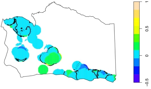
Figure 5 highlights the regions in Santa Barbara County where the difference between the proportion of violations for β=0 and β>0 ambulance responses exceeds 5%, within a distance λ of 4km. The regions within these contours all have a statistically significantly greater proportion of violations for calls where β>0 than calls where β=0. Hence, Figure 5suggests that these highlighted locations, especially areas in central Santa Barbara County, such as Solvang and Santa Ynez, may represent areas where ambulance response time appears to be significantly more sensitive to system load than elsewhere.
DISCUSSION
Our statistical analysis of Santa Barbara County ambulance response in 2006 indicates a significant effect of load on violation frequency. For calls which were preceded by at least one other call within the previous hour and within 20 km, the proportion that are violations is 4.56% compared with 2.96% for calls without such predecessors. The effect of preceding calls seems to be especially pronounced during busy morning and evening commuting hours, whereas during the very early morning (2–5 am), the effect is slightly reversed. The impact of system load is also seen in the fact that the violations themselves are significantly clustered, even after accounting for clustering due to population inhomogeneity. Indeed, at a scale of 0–3 km, it appears that violations are significantly more clustered than one would expect if these calls were a random sampling from all calls. The effect of load on the frequency of response-time exceedances appears to be especially pronounced within semi-rural neighborhoods in central Santa Barbara County, such as Solvang and Santa Ynez.
This study does not attempt to address specific causes for underperformance during system load. Further investigation is necessary to determine what methods may be used to improve response in underperforming areas and to determine how best to implement those improvements. In addition, we did not explore variables that may be confounded with system load and response, such as inclement weather or dangerous traffic conditions. Santa Barbara County is a somewhat unique blend of urban and rural neighborhoods, with few locations of extremely high population density and also few locations that are extremely far from any urban neighborhood. Extension of the present analysis to larger domains and to domains other than Santa Barbara County are important directions for future work.
Footnotes
The authors would like to thank Santa Barbara’s EMS agency and the UCLA EMS study group, especially Jan de Leeuw, Hai Nguyen, Ryan Rosario, and David Zes, for their help in sharing, interpreting, and initial processing of the data.
Supervising Section Editor: Colleen Buono, MD
Submission history: Submitted October 20, 2007; Revision Received August 24, 2008; Accepted November 17, 2008.
Full text available through open access at http://escholarship.org/uc/uciem_westjem
Address for Correspondence: Frederic Paik Schoenberg, ScB, PhD. Associate Professor, UCLA Dept. of Statistics, 8142 Math-Science Building, Los Angeles, CA 90095 USA
Email: frederic@stat.ucla.edu
Conflicts of Interest: By the WestJEM article submission agreement, all authors are required to disclose all affiliations, funding sources, and financial or management relationships that could be perceived as potential sources of bias. The authors disclosed none.
REFERENCES
1. The American Heart Association in collaboration with the International Liaison Committee on Resuscitation. Guidelines 2000 for cardiopulmonary resuscitation and emergency cardiovascular care. Part 12: from science to survival: strengthening the chain of survival in every community. Circulation. 2000;102:I358–I370. [PubMed]
2. Brison RJ, Davidson JR, Dreyer JF, Jones G, Maloney J, Munkley DP, O’Connor HM, Rowe BH. Cardiac arrest in Ontario: circumstances, community response, role of prehospital defibrillation and predictors of survival. Canadian Medical Association Journal. 1992;147:191–199. [PMC free article] [PubMed]
3. Stiell IG, Nesbitt LP, Pickett W, Munkley D, Spaite DW, Banek J, Field B, Luinstra-Toohey L, Maloney J, Dreyer J, Lyver M, Campeau T, Wells G. The OPALS major trauma study: Impact of advanced life support on survival and morbidity. CMAJ.2008;178:1141–1152. [PMC free article] [PubMed]
4. Larsen MP, Eisenberg MS, Cummins RO, Hallstrom AP. Predicting survival from out-of-hospital cardiac arrest: a graphic model. Annals of Emergency Medicine. 1993;22:1652–1658. [PubMed]
5. Blackwell TH, Kaufman JS. Response time effectiveness: comparison of response time and survival in an urban emergency medical services system. Academic Emergency Medicine. 2002;9:288. [PubMed]
6. Fiedler MD, Jones LM, Miller SF, Finley RK. A correlation of response time and results of abdominal gunshot wounds. Archives of Surgery. 1986;121:902–904. [PubMed]
7. Feero S, Hedges JR, Simmons E, Irwin L. Does out-of-hospital EMS time affect trauma survival? . American Journal of Emergency Medicine. 1995;13:133–135. [PubMed]
8. Scott DW, Factor LE, Gorry GA. Predicting the response time of an urban ambulance system. Health Serv Res. 1978;13:404–417. [PMC free article] [PubMed]
9. Fitzsimmons JA. A methodology for emergency ambulance deployment. Management Science. 1973;19:627–636.
10. Ho J, Casey B. Time saved with use of emergency warning lights and sirens during response to requests for emergency medical aid in an urban environment. Annals of Emergency Medicine. 1998;32:585–588. [PubMed]
11. Silverman BW. Density Estimation. London: Chapman and Hall; 1986.
12. Ripley BD. Statistical Inference for Spatial Processes. Cambridge: Cambridge University Press; 1988.
13. Cressie N. Statistics for Spatial Data. New York, NY: John Wiley and Sons, Inc; 1993.
14. Montgomery D, Peck E, Vining GG. Introduction to Linear Regression Analysis. 3rd ed. New York, NY: John Wiley and Sons, Inc; 2001.
15. Baddeley A, Møller J, Waagepetersen R. Non-and semi-parametric estimation of interaction in inhomogeneous point patterns. Statistica Neerlandica. 2000;54:329–350.
16. Veen A, Schoenberg FP. Assessing spatial point process models using weighted K-functions: analysis of California earthquakes. In: Baddeley A, Gregori P, Mateu J, Stoica R, Stoyan D, editors. Lecture Notes in Statistics. New York, NY: Springer; 2005. pp. 269–297.
17. R Development Core Team. R: A Language and Environment for Statistical Computing. Vienna, Austria: R Foundation for Statistical Computing; 2007.
18. Holm S. A simple sequentially rejective multiple test procedure. Scandinavian Journal of Statistics. 1979;6:65–67.